Monitor.sns.gov

• Web Monitor
• Configuring single crystal slices

Web Monitor

To monitor your experiment go to the website monitor.sns.gov

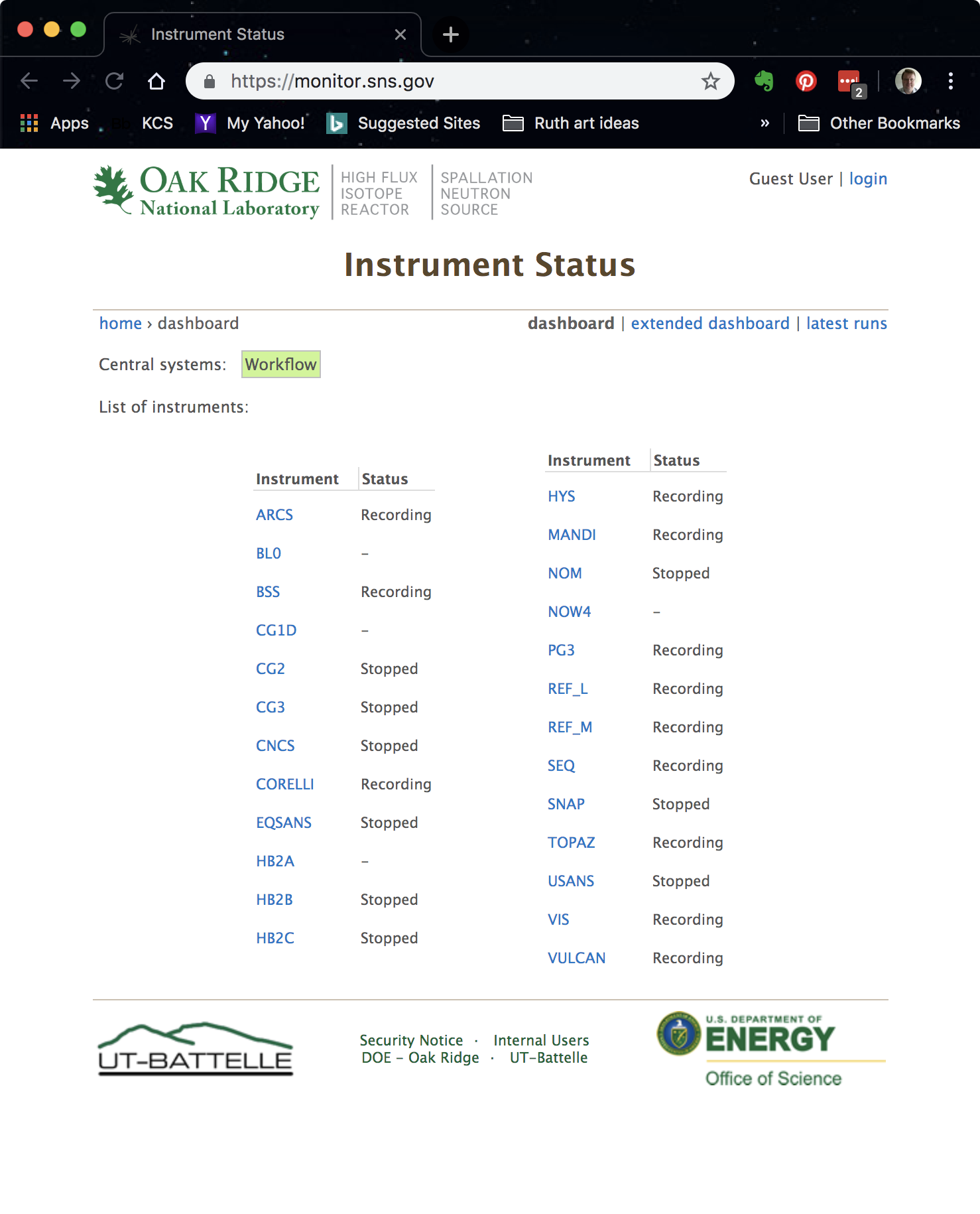
Then select your instrument in this case ARCS.

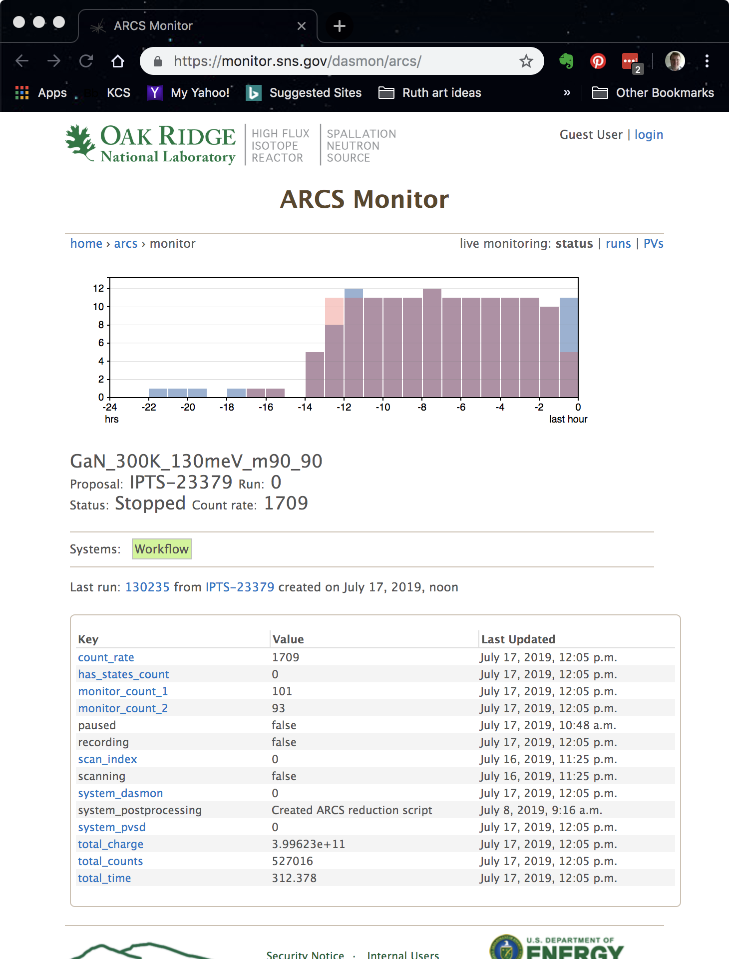Figure 2. the main monitor page for the ARCS instrument

On this page you see what is currently running on the instrument. The graph at the top shows how many files were successfully processed through the saving -> reduction -> cataloging workflow. Red indicates there were errors. These errors can be investigated more thoroughly by clicking on the runs link in the right.

The Runs link takes the user to a list of runs in the current IPTS as shown in Figure 3. If you want to see a different experiment simply replace the number in the hyperlink with the desired proposal.

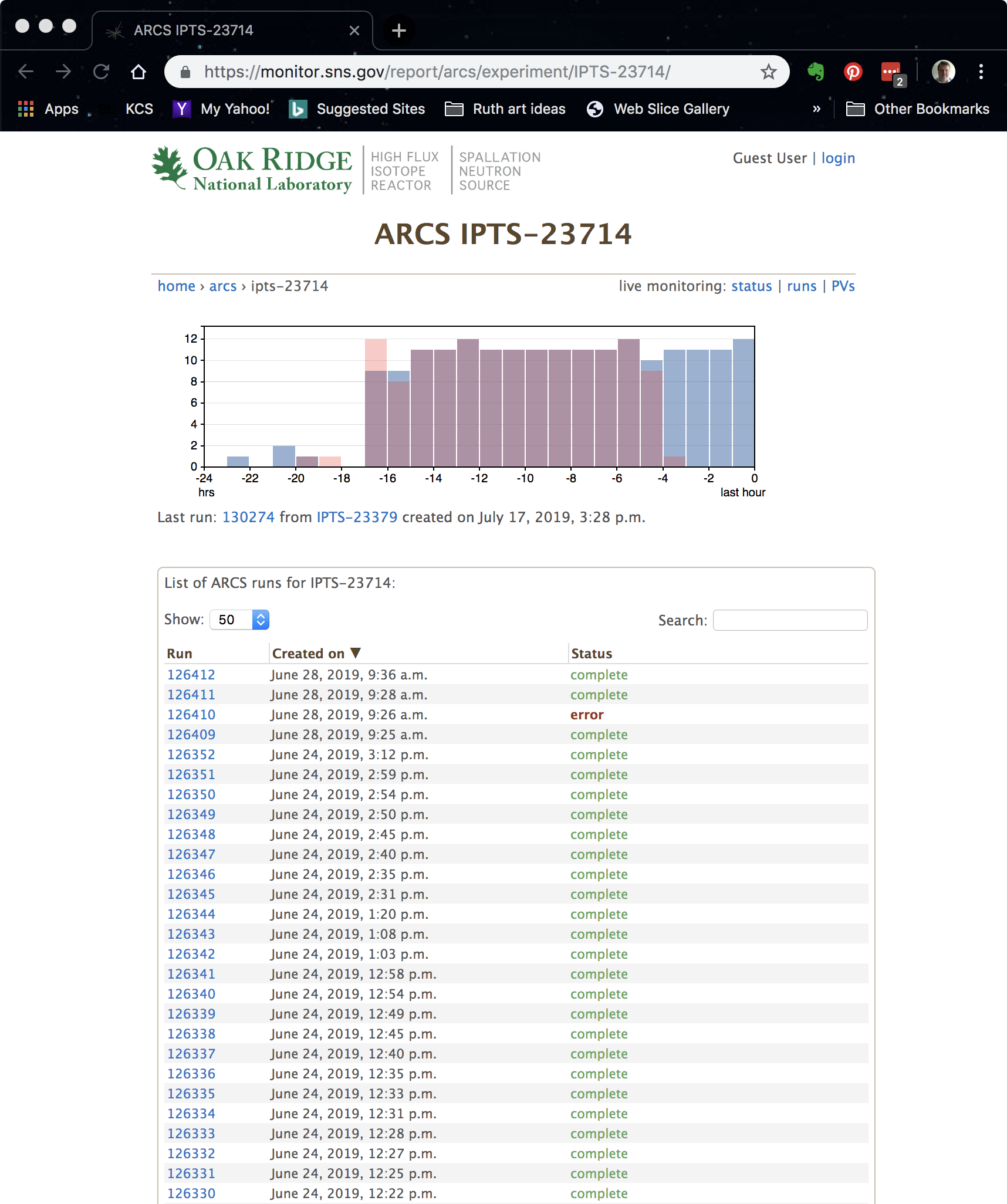Figure 3. the Runs view from monitor.sns.gov

Alternatively the PVs link allows the user to examine the status of various metadata variables as shown in Figure 4.

If the user clicks on any PV, for example BL18:SE:SampleTemp A window showing the last fiew minutes of that log value are shown.

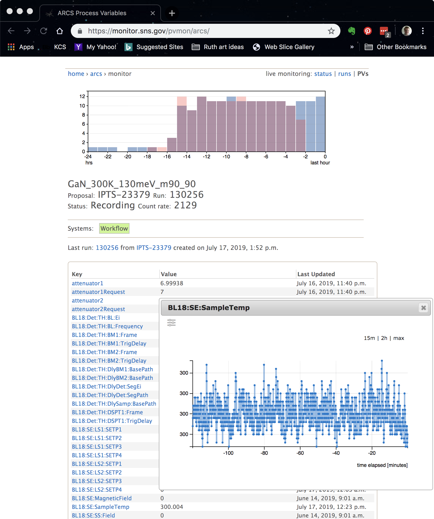
Figure 4. A view of the web monitor after the sample temperature link is selected.

If you are a user for the IPTS on the runs view in Figure 3, you can click on a run to see more information. In order to verify you are on the proposal you need to login with your XCAMS user name and password using the login link in the upper right.

Once logged in you will see a view like in Figure 5.

• The title and some preliminary information are at the Top
• A view of the autoreduced data is on the screen. If you hover over the data you will see a tool bar that will allow you to zoom and do other simple manipulations to the data.

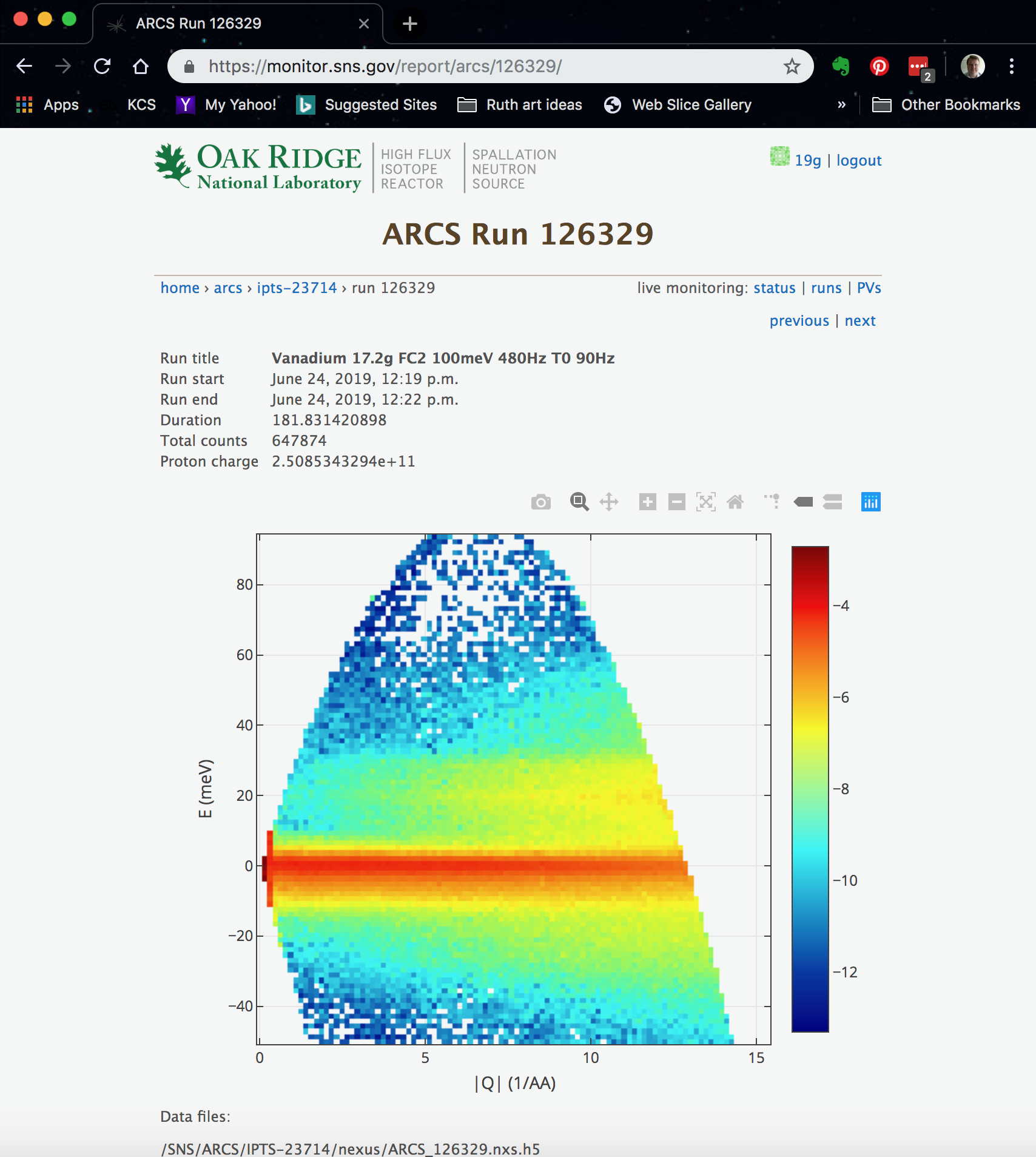
Figure 5.

Configuring single crystal slices

monitor.sns.gov can display slices of rotation sets. The sets are defined by all files with the same sequence name

To start this on an analysis machine,

1. go to the shared/autoreduce directory in your IPTS directory

2. execute the autoreduction_plotting_setup.sh script by typing

   ./autoreduction_plotting_setup.sh

   or

   source ./autoreduction_plotting_setup.sh

   The gui in Figure 6. will open up where you can define your slices

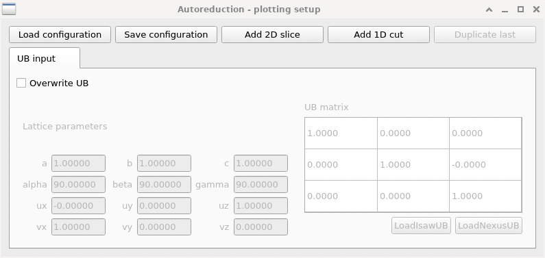   Figure 6.

3. If you need to set a UB to something other than is in the NeXus file, use the UB input tab by clicking the Overwrite UB check box as shown in Figure 7. Note that this only overwrites the UB for the displayed.

   
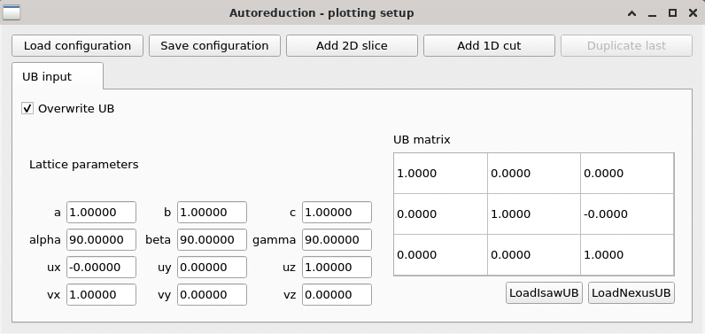
   Figure 7.

4. Select add 2D slice or add 1D cut to generate one or the other. AN example of the box to fill in for a 2D slice is shown in Figure 8.

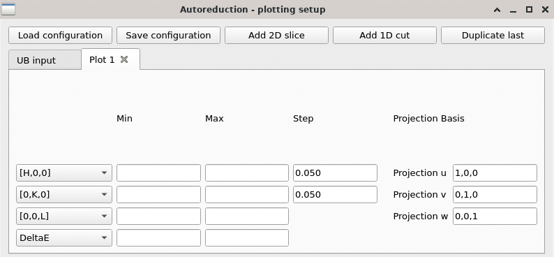   Figure 8.

5. Fill in the boxes

6. Select another add a slice or a cut to add more slcies or cuts. The “duplicate last” will duplicate the parameters in the last cut or slice. This allows you to quickly build up a set a of relevant slices or cuts.

7. Once the cuts and slices are all set up press “save configuration” as shown in Figure 9.

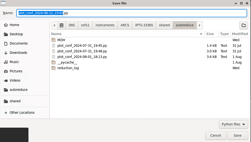   Figure 9.

8. Simply hit the “save” button. Do not change the file name or the path to the file. The auto reduction script looks for the the most recent file to know how to generate cuts

9. If you already have a saved configuration and need to add another slice or cut use the “load configuration” to load the old configuration of slices as shown in Figure 10. Note that the additional slice will only start from the current file that is in use. 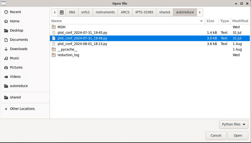Figure 10.

A result of a load configuration showing multiple slices is shown in Figure 11.

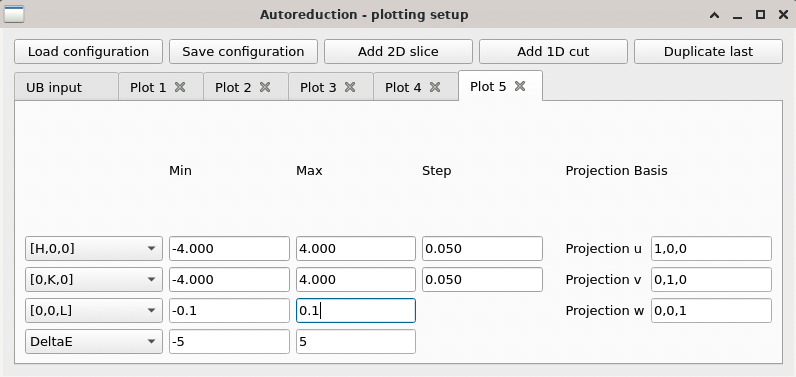Figure 11.