Visualization tools

• Shiver for single crystal visualization
• Mantid
  • mslice for powder reduction
• Dave
  • Getting Started with DAVE-Mslice for use at SNS
  • Powder data with DAVE-Mslice

This describes software that is used for visualization of your data acquired on the DGS instruments. We expect that you will primarily use the machines at analysis.sns.gov.

Shiver for single crystal visualization

The recommended way to visualize single crystal data is using Shiver, which is a gui and scripting tool that leverages Mantid and its multidimensional data structures and algorithms. Documentation on how to use Shiver can be found the Shiver github pages site

Mantid

1. Log into analysis.sns.gov

2. Open a terminal by right clicking on the desktop and selecting “Open in Terminal”.

3. Type mantidworkbench at the command line prompt and press the Enter key. (If your local contact suggests it or if you want to use the newest features in Mantid type mantidworkbench nightly)

4. This will open the main mantidworkbench window shown in Figure 1.

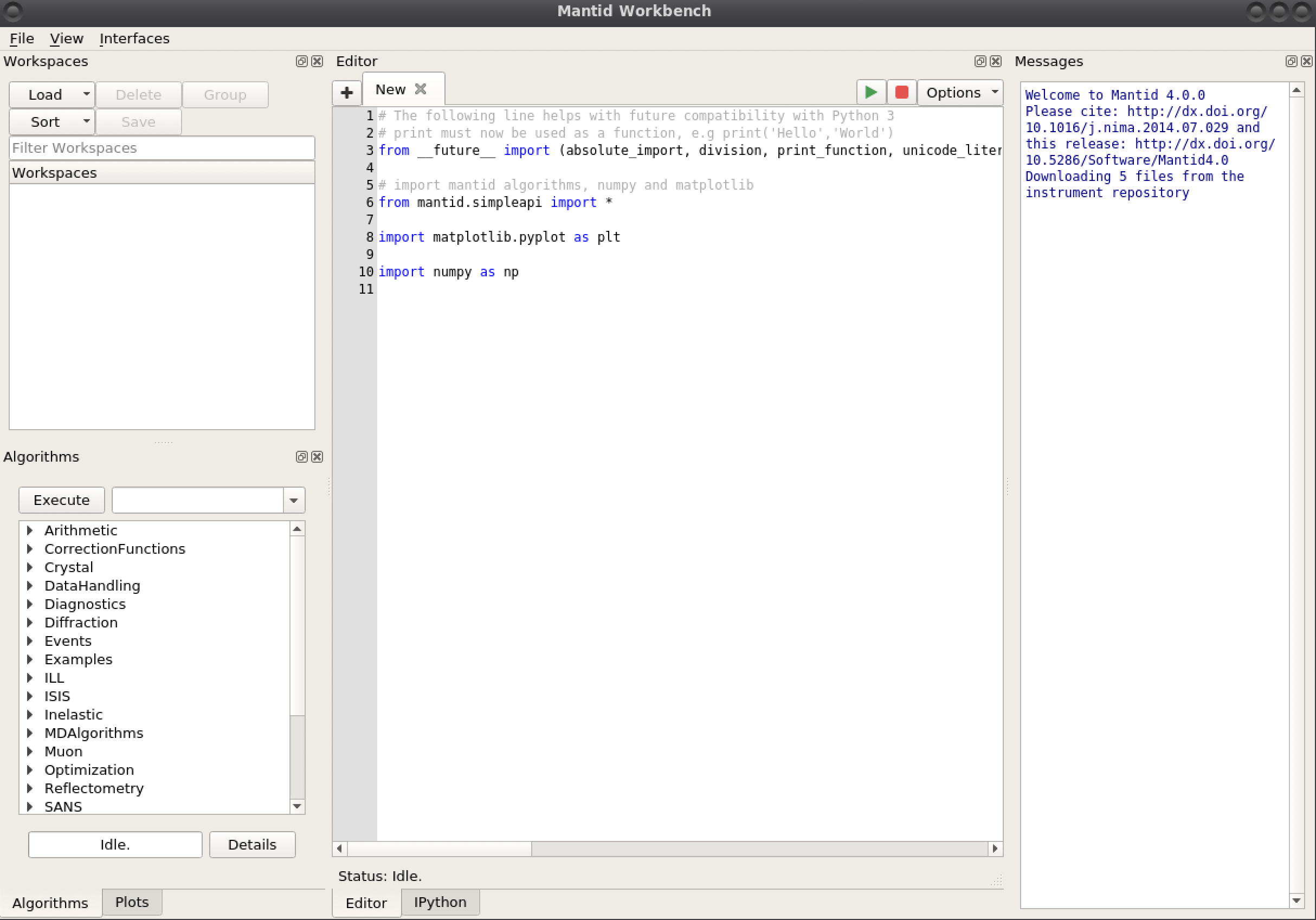Figure 1. The main Mantid Workbench window

mslice for powder reduction

1. Click on Interfaces on the top menu and choose Direct, then choose MSlice. as shown in Figure 2.

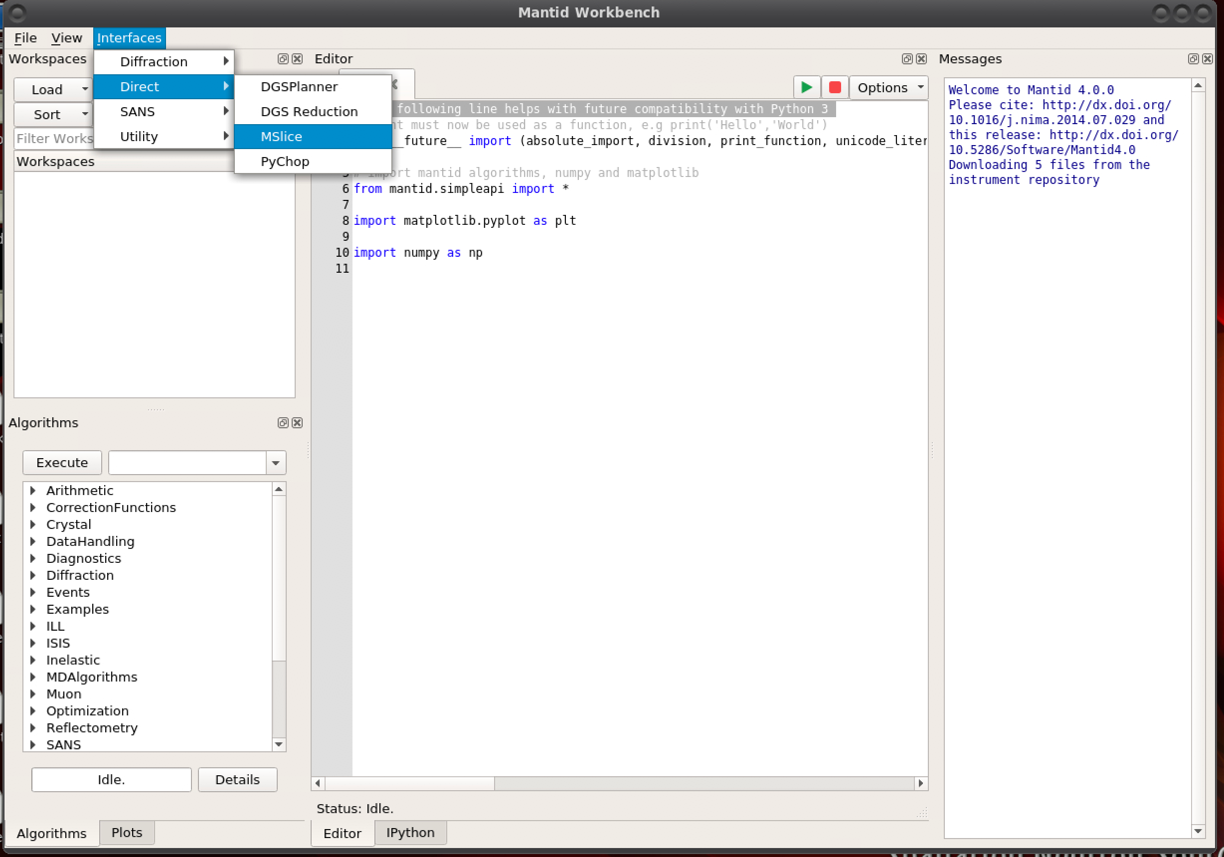Figure 2. Starting Mslice from the Mantid workbench

The above steps launch the Mantid mslice file and workspace management window shown in Figure 3.

• Notice there is a Data Loading Tab that allows you to load new data into a workspace.

• There is a Workspce Manager Tab to allow the user to view the workspaces that are in memory.
• Finally there is an ipython terminal window at the bottom to allow the user to script or perform additional functionality not available in the gui.

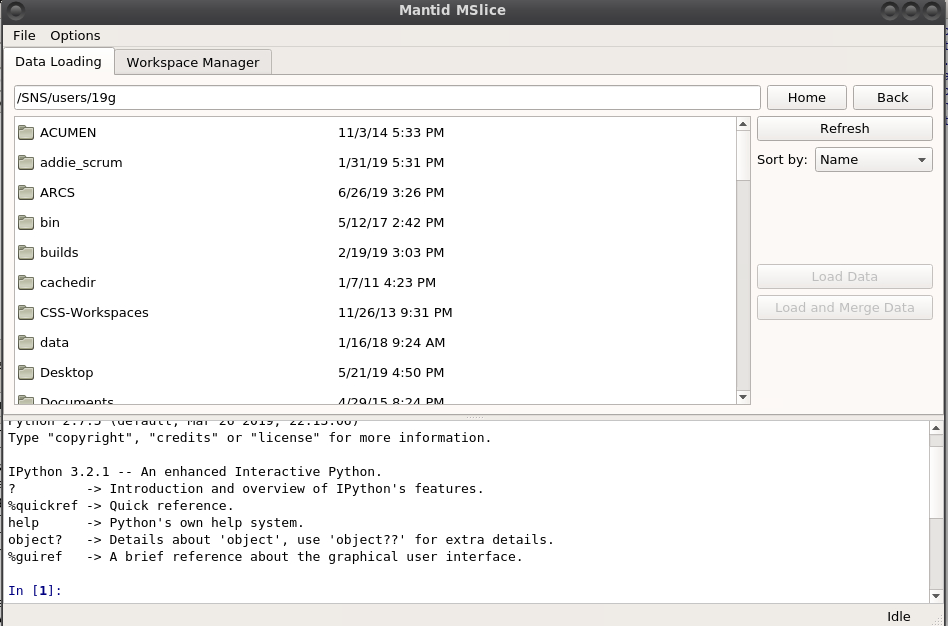Figure 3. The Mantid mslice file and workspace management window

1. Load data into a new workspace

• From the Data Loading tab browse to your data file and then click on Load Data. Typically you want an .nxspe file.

• The data will typically be locaed in a directory /SNS/snfs1/instruments/SEQ/IPTS-NNNNN/shared/autoreduce/ where NNNNN is the IPTS number of your experiment.

• An identical location (a symbolic link) of the data is at /users/XYZ/data/SNS/ABC/IPTS-NNNNN/shared/autoreduce/ where XYZ is your UCAMS or XCAMS identification, ABC is the instrument used for the measurement (SEQ, ARCS, CNCS, or HYS), and NNNNN is the IPTS number. Some instruments generate a powder averaged nxspe data file that would be located in an additional subdirectory. The powder averaged .nxspe files are much smaller in size, and will load faster.

1. Calculate Projections

• When the data is loaded into a workspace the workspace tab is automatically selected and you see the view in Figure 4.
• If the data has already been powder averaged, the powder tab will be greyed out.

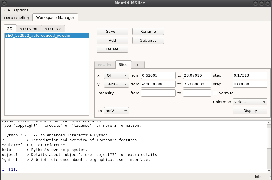Figure 4. The Slice and Cut view of the Mslice window

1. Plot a slice

• Choose your preferred viewing axes in the x and y boxes.
• Choose the from, to and step size for each axis.
• Note that these values are automatically filled in.
• Then click Display

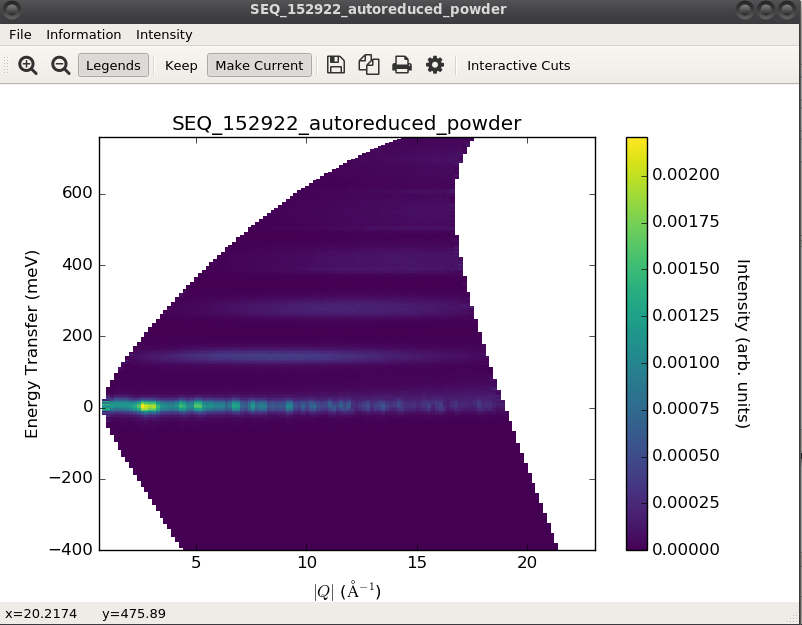Figure 5 an Example slice using the default parameters

• To adjust the look of the plot click on the plot options button on the menu bar as shown in Figure 6.

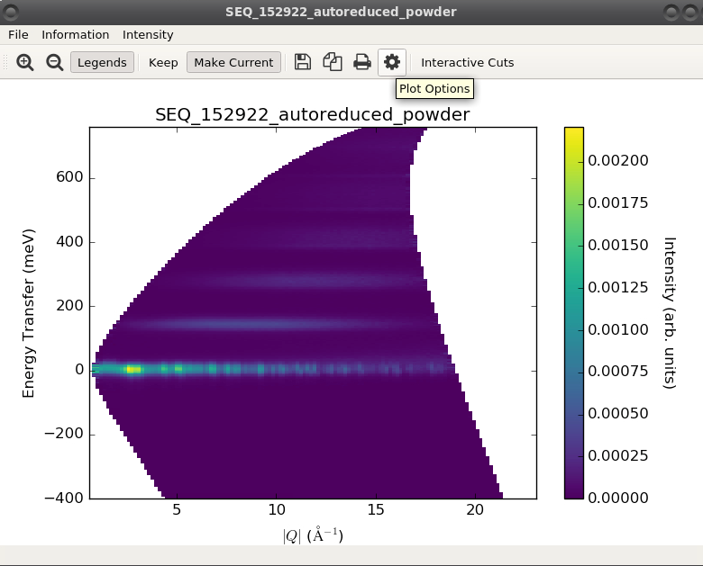Figure 6. The plot options button.

• The plot options window is shown in Figure 7. It shows how you can make cosmetic changes to plots. For example Changing the yaxis minimum and the maximum on the color scale provides Figure 8.

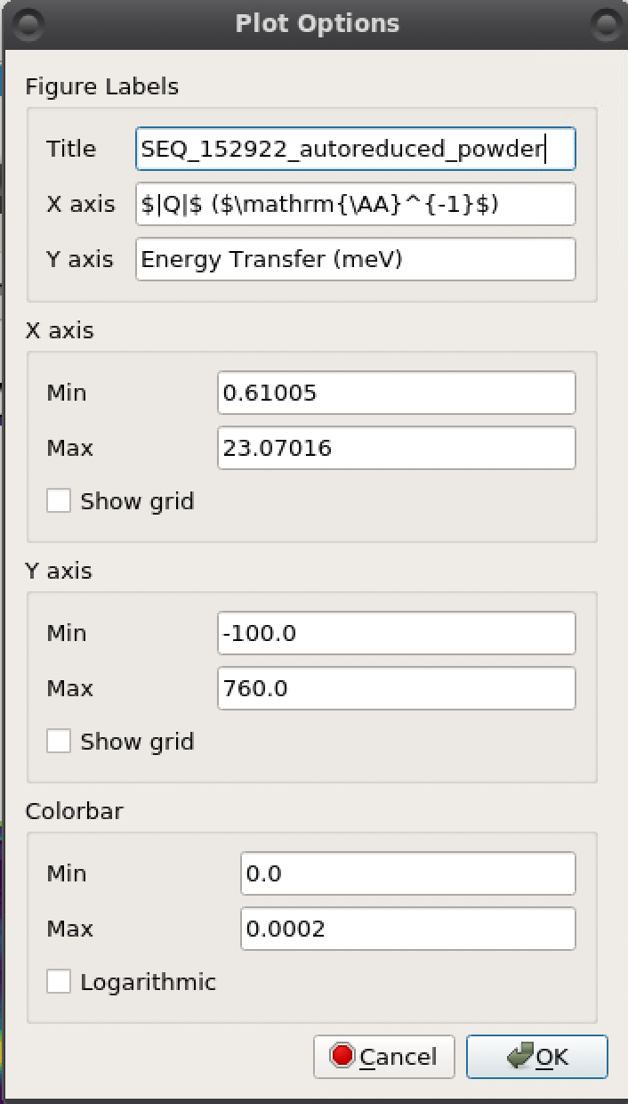Figure 7. The window

• if you want to keep the plot for comaprison, click the keep button. Otherwise the next figure generated will be in this window.

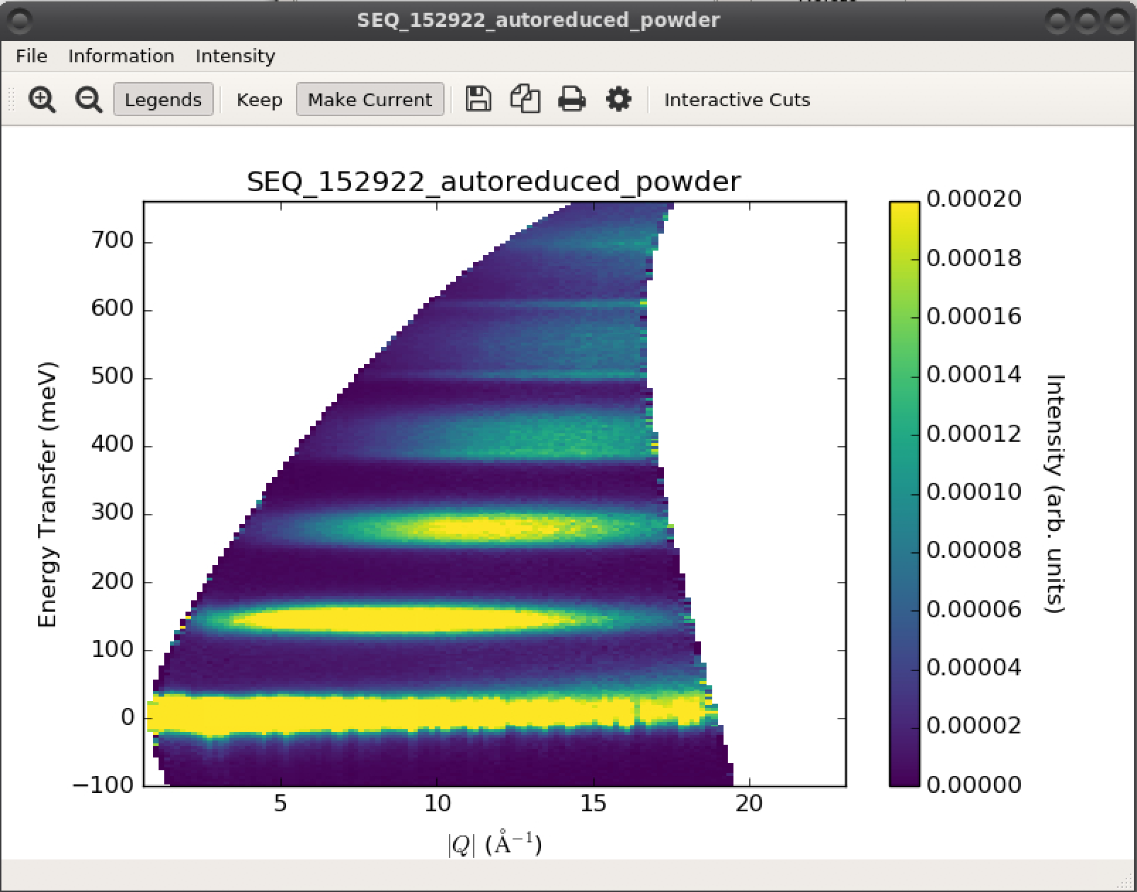Figure 8. Same plot as in figure 6 with the color intensity and the yaxis limits adjusted.

1. Plot a Cut

To plot a cut:

• select the Cut Tab from the Mslice window shown in Figure 4. The Window should look like Figure 9.
• Next select which direction to cut along using the along pulldown. Then reference a slice (Figure 8) to determine where you want to cut. fill in the From, to, step

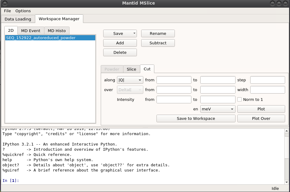Figure 9, the Main Mantid window with the Cut tab selected.

• Figure 10 shows the cut tab with some values selected.

• Press plot to generate the figure in the current plot window.

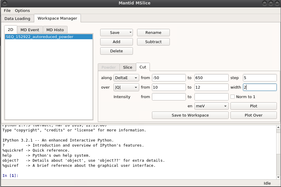Figure 10. The mslice window with the Cut tab filled in

The resultant cut is shown in figure 11.

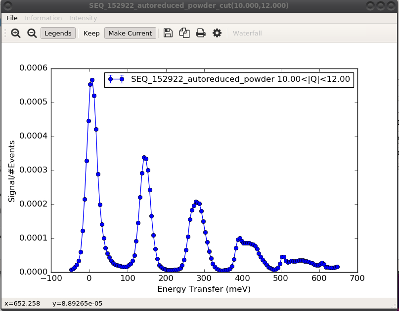Figure 11.

Dave

DAVE-Mslice is available from the DAVE (Data Analysis sand Visualization Environment) website at https://www.ncnr.nist.gov/dave/ The Mslice GUI is a package available from within DAVE.

Getting Started with DAVE-Mslice for use at SNS

1. Log into analysis.sns.gov

2. Open a terminal by right clicking on the desktop and selecting “Open in Terminal”.

3. Type dave at the command line prompt and press the Enter key.

4. This will open the main DAVE window shown in Figure 1.

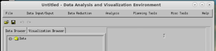Figure 1. Top of the main DAVE window

1. Click on Data Reduction on the top menu and choose NCNR, then choose DCS Reduction (Mslice) as shown in Figure 2.

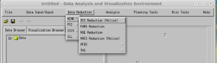Figure 2. Choosing the DCS Reduction (Mslice) option from the main DAVE window.

1. The Mslice window will appear as shown in Figure 3. This window is divided into three panels. The top panel is for loading data. The middle panel is for projecting data into different coordinate systems, and the bottom panel is for plotting data. Additional options are available from the pulldown menus at the top of the window. The next sections describe the steps to load, project and plot powder data.

Powder data with DAVE-Mslice

1. Load the data.

• DAVE-Mslice will only indicate available files of the File Type chosen in the file menu at the top left of the DAVE-Mslice window. Click on the File pulldown menu, then choose File Type, then choose the NXSPE file type.

• Navigate to the data directory. Use the box on the left of the top panel of the DAVE-Mslice window as shown in Figure 3 to navigate to the directory of the data you wish to load. This directory will typically be at a location such as /SNS/snfs1/instruments/SEQ/IPTS-NNNNN/shared/autoreduce/ where NNNNN is the IPTS number of your experiment.

• An identical location (a symbolic link) of the data is at /users/XYZ/data/SNS/ABC/IPTS-NNNNN/shared/autoreduce/ where XYZ is your UCAMS or XCAMS identification, ABC is the instrument used for the measurement (SEQ, ARCS, CNCS, or HYS), and NNNNN is the IPTS number. Some instruments generate a powder averaged nxspe data file that would be located in an additional subdirectory. The powder averaged .nxspe files are much smaller in size, and will load faster.

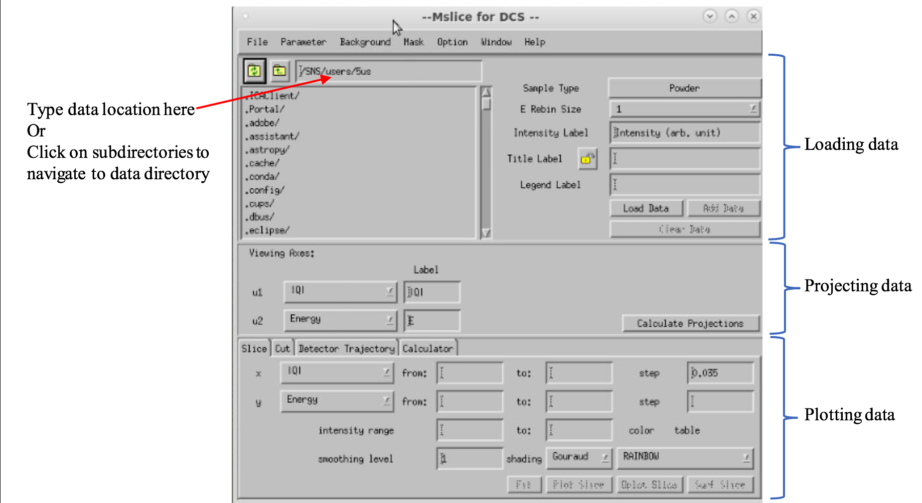Figure 3. The DAVE-Mslice window. The window is shown for Powder Sample Types.

• In the Loading data panel, verify that the Sample Type is chosen as Powder. This is a pulldown menu in the upper right portion of the top panel.

• In the list of files available, click on the files or group of files that you would like to load. Use the Shift key in combination with clicking to load non-continuous files from the list. See Figure 4. Loading multiple files will average the data together. This averaging will not take into account different count times or proton charge accumulation times used for the measurements. You may need to average datafiles together using appropriate mantidplot commands prior to loading them with DAVE-Mslice to account properly for counting statistics.

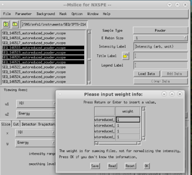Figure 4. DAVE-Mslice window when loading data files.

• Click Load Data button in the top panel. A dialog box will be displayed asking for the “input weight” of each file that is loaded. If all of your data have been normalized to the same proton charge, you can keep the value of 1 in each of these cells and click OK. This is very often the case. The data will then load.

• If you have already loaded a set of data, and you wish to average another file with this group, you may highlight that file and click Add Data. Note that this does not account for different count times/proton charge accumulated for each measurement.

1. Project the data. Choose which coordinate system in which you would like to project your data using the pulldown menus to the left of the Projecting data panel. As shown in Figure 3, the default coordinates are |Q| and Energy. Another often used option for the coordinate system for powder data are 2Theta and Energy.

2. Plot the data. Powder data can be plotted as a slice (two-dimensional data, or intensity as a function of two independent variables) or a cut (one-dimensional data, or intensity as a function of one independent variable).

• For a slice of data, one first chooses the Slice tab at the bottom of the DAVE-Mslice window. Then one chooses the x and y coordinates from the pull-down menus on the left of the bottom panel of the DAVE-Mslice window as shown in Figure 3. If the from and to values are not entered, the plot will be made over the entire range of that variable. If the step value is not entered, the minimum step size allowed in the data will be used. If values are not set in the intensity range, the range of the figure will be set based upon the maximum and minimum intensity values. The smoothing level applies a Gaussian approximation smoothing kernel to the data N times, where N is the smoothing level. The smoothing kernel can be changed in the Parameter menu. Warning smoothing is to help with visualizing only. Do not smooth slices that will be used in subsequent analysis. Many choices are available in the color table pulldown menu in the plotting panel. Clicking Plot Slice will plot the slice. The intensity, x-axis, y-axis scales and color table can also be changed directly from a figure after it is plotted. After a slice is generated, one can cut through this slice dynamically by right clicking on the slice and choosing Cut and then choosing the cut direction. Warning The error bars and intensity values are potentially interpolated values in this cut. For Quantitative use of a cut use the cut tab as described below.

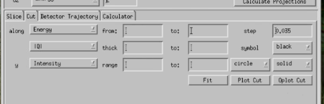Figure 5. Plotting panel of the DAVE-Mslice application with the Cut tab selected

• For a cut of data, one chooses the Cut tab at the bottom of the DAVE-Mslice window. Then one chooses along which independent variable the cut is being made using the along pull-down menu. If the from and to values are not entered, the plot will be made over the entire range of that variable. If the step value is not entered, the minimum step size allowed in the data will be used. The range of integration of the other independent variable can be set using the next line in the window. The intensity range and binning can also be adjusted. The type of plot symbols, plot line, and color can be adjusted. One then clicks on Plot Cut or one can overplot the data on the current figure with the Oplot option. Figure 5 shows the Cut tab of the plotting panel in DAVE-Mslice. The Fit button allows one to do simple fits using the PAN: Peak Analysis tool in DAVE.

• After figures are generated, many figure details including titles and logarithmic and linear axes can be adjusted by double clicking on the figure elements and making changes.

• Using the Keep pull-down menu in a figure window will keep that figure on the desktop and prevent it from being overwritten. The Make Current menu in a figure window will make the figure active again for over-plotting or plotting data.

1. Often used options

• Background subtraction - A Background can be subtracted from the data by selecting data files in a similar manner as loading the data, but then clicking on the Background menu and selecting Load Empty Can File(s). The background subtraction can be halted by choosing Clear Background in the Background pull-down menu. A self-shielding factor, a multiplicative factor applied to the Background data before it is subtracted, can be adjusted by clicking on the Change Self-shielding Factor… option under the Parameter pull down menu. The Self-Shielding factor should be less than or equal to 1.

• The Option pull down menu provides routines for simple data manipulation. Some common choices are:

• Powder line locations of common sample can materials can be overplotted using the Show Powder Line option.

• If the elastic peak position is shifted by a small percentage, the Elastic Peak Position Adjustment option can be used. Warning because of the asymmetric peak shape on ARCS and SEQUOIA, the center of mass of the peak is not at the same location as the maximum in the peak.

• The data can be viewed in different formats including χ(Q,ω) and two different density of states formats using the View Intensity As option.

• Simple Absorption corrections can be performed with the Absorption Correction option. Calculations of the variables for this option can be performed using the Planning Tools menu of the main Dave window shown in Figure 1.

1. Exporting data – Once a cut or a slice has been generated, you can save the figure in several image formats using the File->Save Plot As submenu on the particular figure that is being saved. You are also able to save the numerical values of the most recently plotted cut or slice from the File pull down menu of the main DAVE-Mslice window. Choose File -> Save Slice Data as OR File-> Save Cut Data as for the corresponding data you wish to save. Several data formats are available for the saved data files.